Performing Like An Algorithm
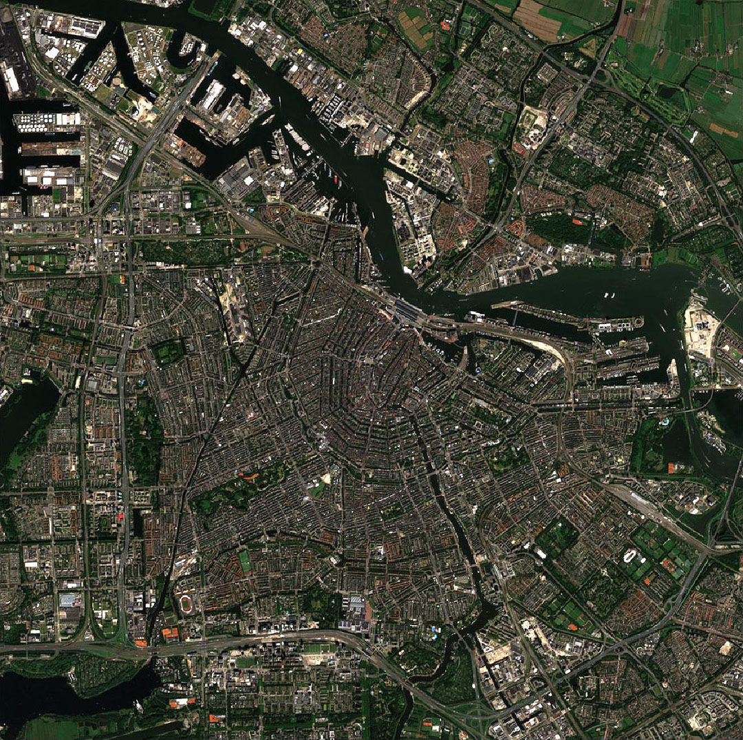
As in the real-time version, the results are produced from bona fide geospatial data: from the European Space Agency's Sentinel-2 satellites for the unsupervised learning algorithm and the large pretrained neural networks, while several of the smaller models operate on data from Planet Labs SuperDove satellites.
In all cases, the categorized classes appear as graphical objects. However, the classification process establishes artificial boundaries, implying landscapes that are more organized than they in fact are. These artifacts, coupled with colorization for readability and their integration into GeoAI systems, further contribute to fabrication tendencies long acknowledged in map-making.
Unsupervised Clustering
K-means
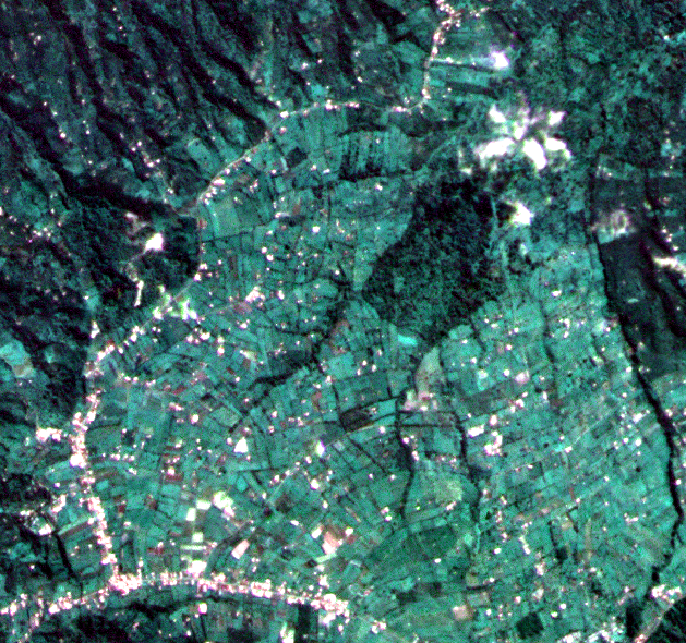
Clustering works without instructions on the input data. It simply finds similarities in datasets and arranges them into groups. Because it can do this operation without knowing anything about the data, it is considered an unsupervised learning approach. Centroid-based clustering places reference points randomly within a data collection and iteratively moves those points around, minimizing the overall distance between those reference points and the data. Almost magically, order emerges and patterns appear. Clustering, and the k-means variant used here, does not need human guidance and can find things that might surprise us, as the examples below will illustrate.
Select a site
How many different categories do you want to generate?
Arithmetic Operators
Normalized Difference Vegetation Index
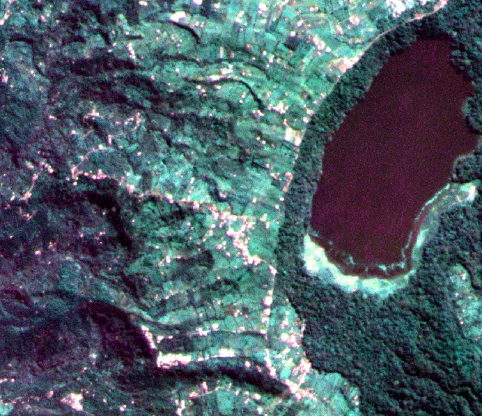
The Normalized Difference Vegetation Index (NDVI) is a widely employed metric in GeoAI for estimating the density of vegetation on land. It involves a straightforward arithmetic calculation using the red and near-infrared bands. Like k-means, it is an unsupervised approach and does not require training data. For that reason, NDVI and similar arithmetic operations are appealing for land surveys. However, these convenient operators have limitations.
Select a site
Supervised Learning
Supervised machine learning algorithms use data to train models. They learn the characteristics of target classes from training samples to identify these learned characteristics in new datasets. Some learning algorithms produce smaller models with fewer internal parameters and require smaller training sets than others. Many of them have been in use for a long time. I refer to these learning machines as old-guard learning machines for that reason. This class includes Random Forest, Support Vector Machine, and shallow neural networks. GeoAI has relied on these classifiers for decades for land cover analysis.
Creating a high-quality dataset is key to model performance. The training process depends on representative samples that cover the distribution of the desired categories. If the chosen samples are inadequate or the dataset is too small, the classification results will be compromised. Complex data categories, such as agroforestry and rice paddies, present serious challenges for machine learning systems. The recent success of image classification owes much to well-organized training data applied to well-defined categories. When algorithms are trained and tested on such well-structured datasets, they can effectively discriminate between objects. Differentiating between cars, trains, and airplanes, for example, is a relatively straightforward task. Even discerning between similar-looking car models poses no problem for a well-designed classifier. Automobiles do not shape-shift. They are uniform and predictable compared to agroforestry plots.
Random Forest
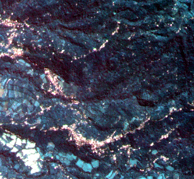
The Random Forest classifier (RF) is a classic. The term forest stems from the fact that the classifier orchestrates an ensemble of simpler base elements, decision trees. The algorithm randomly divides up a given dataset into chunks, a process called bagging, and distributes these chunks to its ensemble of decision trees. Once the individual trees have come to their respective conclusions, RF, when it operates as a classifier, lets these trees “vote for the most popular class.” The class with the most votes wins and becomes the classification result. Each time you train an RF, you get a different result, though the differences are often small.
RF is widely employed in remote sensing due to the accuracy of its classifications and the comparative simplicity of the underlying algorithm. But how will RF respond to the complex land cover features of the Alas Mertajati?
Select a site
Support Vector Machine
The Support Vector Machine (SVM) algorithm separates data into different classes by finding an optimal dividing line between given sets. In two dimensions, this process is easy to visualize. Picture a set of red dots on one side of a page and a set of blue points on the other side. You can position a straight line on the page “just so” to maximize the distance between the line and each set of dots. However, when dealing with non-linear data that cannot be separated by a straight line in a two-dimensional space, a different approach is required. In higher dimensions, a hyperplane replaces the line, becoming a surface in two dimensions, for example. SVM utilizes a technique called the kernel trick to operate in higher-dimensional feature spaces without the need to compute the data's coordinates in those spaces. This makes SVM an efficient classification machine. In the realm of GeoAI analysis, SVM is a core component due to its ability to efficiently handle multi-class classification, which aligns perfectly with our requirements. However, SVM can perform poorly when data features are vague and overlapping, as is the case in the Alas Mertajati land cover dataset.
Select a site
Neural networks
Neural Networks (NN), loosely inspired by biological neural networks, consist of interconnected nodes that store and transmit data. Each node's signal strength, controlled by assigned weights, influences subsequent layers. Typically, NNs include an input layer receiving external data such as an image, an output layer providing the network's response, and intermediate layers across which the data flows. During operation, an objective function calculates the difference between current and desired outputs. The network adjusts its internal parameters to minimize this difference until a stopping criterion is met.
U-Net
Neural network–based approaches such as U-Net constitute the newest and largest class of machine learning systems for landscape analysis. As in other fields, such as language translation, speech synthesis, and most recently, text and image generation, NNs have demonstrated superior results. NNs have been so successful at previously challenging tasks that they are now considered candidate material for the ultimate goal of AI, Artificial General Intelligence. For that reason alone, it makes sense to compare NN-based approaches with the smaller models described above.
Residual Networks
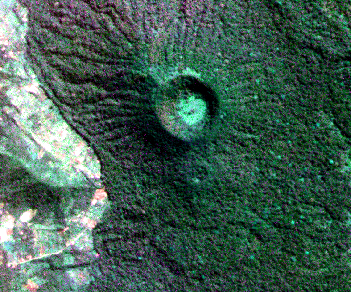
A residual network (ResNet) is an NN-based deep learning architecture that introduces skip connections that allow the model to bypass one or more layers, enabling the training of much deeper networks effectively. This architecture is particularly beneficial for image segmentation tasks, such as land cover analysis, as it captures intricate features and spatial hierarchies in complex images.
The Allen AI Institute's SaTLas ResNet models, trained on terabytes of Sentinel-2 satellite imagery, can respond to a variety of landscape conditions. For example, the category parks captures larger built environment features such as dams, parking, landfill, airports, and power plants. The category power is designed to capture structures such as mine shafts, lighthouses, offshore platforms, and petroleum wells. The collection of categories titled vegetation captures grass, crops, wetlands, mangroves, and trees. The feature set roads captures roads, railways, and runways, and the category agriculture is designed for agricultural production such as rice, corn, sugarcane, wheat, barley, cassava, potato, sunflower, and coffee. Nonetheless, agroforestry remains invisible within the SaTLas representation, highlighting how GeoAI systems can obscure complex, heterogeneous land practices that fall outside standardized categories.
Select a category
Given the radically different approaches deployed by each of these algorithms, it is perhaps surprising that they produce such similar results. The NN is a comparatively shallow model with only two hidden layers. Nonetheless, the NN is able to capture most of the intricacies of the landscape. Overall, however, NN fails, as does RF, to succinctly differentiate agroforestry from forested areas. While the results from SVM and RF are likely as good as they can be, the output of the NN and its U-Net cousin can improve by expanding the network with additional layers. However, that added depth requires more training data and much more compute power, both of which are in short supply for most resource-constrained projects.